3.3. Multiple Dimensions
So far, we have only dealt with the completely scalar case of linear regression. We assumed that \(Y = \theta X + \epsilon\), where \(Y, \theta, X\) were all scalars. However, we often have more than one input feature that contributes to the output. If we might want to base our predictions off of two factors, for example \(Y = \theta_1 X_1 + \theta_2 X_2 + \epsilon\). To gracefully scale to cases where we have two or perhaps hundreds of input features, we need to use some concepts from linear algebra. This section will derive linear regression with multiple dimensions while introducing concepts from linear algebra along the way.
Linear algebra is a way of arguing about multi-dimensional collections of numbers. A vector is just a collection of numbers. Each vector belongs to a vector space, where addition and scalar multiplication are defined in addition to other necessary properties.
3.3.1. The Model & Linear Algebra
Our previous model of the world was \(Y = \theta X + \epsilon\) and our prediction model was \(\hat{y} = \theta x\). We assume that the observed \(Y\) is a function (\(k\)) features and noise:
Our predictive model is then
Rather than using \(k\) different values for \(\theta\), we can express \(\theta\) as a single vector. For example, \(\theta = \begin{bmatrix} \theta_1 \\ \vdots \\ \theta_k \end{bmatrix}\). Each value of \(x\) is then also a vector of the same size \(k\).
Definition: Dot Product
In linear algebra, the quantity \(\theta_1 x_1 + \theta_2 x_2 + ... + \theta_k x_k = \sum_{i=1}^k \theta_i x_i\) is defined as the dot product between two vectors \(\theta\) and \(x\), written as \(\theta \cdot x\). Once we define basic matrix multiplication, we can also write the dot product as \(\theta^\top x\). In matrix multiplication, the \(i\)th row of the left is “dot-product“‘d with the \(j\) column of the right item. “\(\top\)” means transpose, or that we swap the rows with columns.
Thus, our model just becomes the dot product between two vectors. We can use the exact same derivation as the 1D case except replace \(\theta x\) with \(\theta^T x\). So the multi-dimensional optimization problem is as follows.
Some of you might notice that this equation also seems to have the form of a dot product! Specifically, a dot product between a vector of all of the errors from the entire dataset and itself. Though we could write this as a vector with all of the individual components, its easier to write this as a matrix multiplication. Let’s examine how we can write the vector of errors.
\(X\) is an \(N \times k\) matrix, where each row is one of the \(N\) total data points in the training set. It’s commonly referred to as the data matrix
\(X\theta\) is a vector of our predictions as the \(i\)th row (data point) is applied to the (only column of) the weight vector to form the \(i\)th output component. We can then reduce the total expression.
Earlier our cost function had a nice interpretation: it was the sum of squared errors. From the current form that’s not entirely clear. One thing we can notice is that when we apply a dot product to the same vector, it gives a measure of distance, referred to as norm. Specifically, \(v^\top v = v_1^2 + \dots + v_k^2\). You may notice that this is the square of the distance of the vector \(v\) from the origin. We refer to this type of distance as the \(l2\)-norm. The dot product we have defined thus induces the \(l2\)-norm. The notation is as follows: \(v^T v = ||v||^2_2\), where the superscript denotes that the quantity is squared, and the subscript denotes the \(l2\)-norm. Other norms will become important later.
This means that our cost function in full fledged vector form can be written as follows:
We can interpret this as minimizing the magnitude of the error vectors. It turns out we can still solve this problem. You may have heard of it being called “Least Squares” regression before.
3.3.2. The Calculus Solution
We can derive the solution analagously with the 1D case. This requires matrix calculus, or techniques for multi-variate calculus applied to matrices. We won’t go into to much detail here, but just know that the gradient of a function \(f: \mathbb{R}^k \rightarrow \mathbb{R}\) is a vector of all of the martial derivatives of the output of the function with respect to the input components. It’s also the transpose of the Jacobian in this case. As cost functions usually output a single scalar value, in machine learning we often only need to use gradients.
By scaling to multiple dimensions, we didn’t change the convexity of the problem, so critical points are still guaranteed to be optimal. We can proceed by taking the gradient of the cost with respect to the weights \(\theta\).
This equality is called the normal equation. It gets this name because it can also be interpreted as a geometric projection.
3.3.2.1. The Geometric Solution
The geometric solution to least squares will help you build some intuition for linear algebra. Our objective has been to minimize the norm of the error: \(\min_\theta ||y - X\theta||\). We can interpret the labels \(y\) as one vector and the predictions \(X\theta\) as another vector. Our optimal solution is when these two vectors are as close together as possible. However, note that the predictions \(X\theta\) are not free to be any vector we want – they are in fact restricted to a set we call the column space of the matrix \(X\).
Definition: Column Space The column space of a matrix \(X\) is the set of all possible linear combinations of the columns of the matrix \(X\) or equivalently the set of all possible vectors \(v\) such that \(v = Xu\) for some \(u\) in the vector space. Assuming our vector space is defined under \(\mathbb{R}^N\):
Note that the column space is (usually) not equal to the entire vector space, meaning we can’t reach every single possible vector using the matrix \(X\). In the context of least squares regression, this makes sense as our model is linear and thus cannot express some complex model. However, we can still try and get as close to the perfect solution as possible using our linear model. In the figure below, the column space of \(X\) is depicted as the plane, and our error vector \(y\) is not on the plane (meaning our data isn’t perfectly linear as expected).
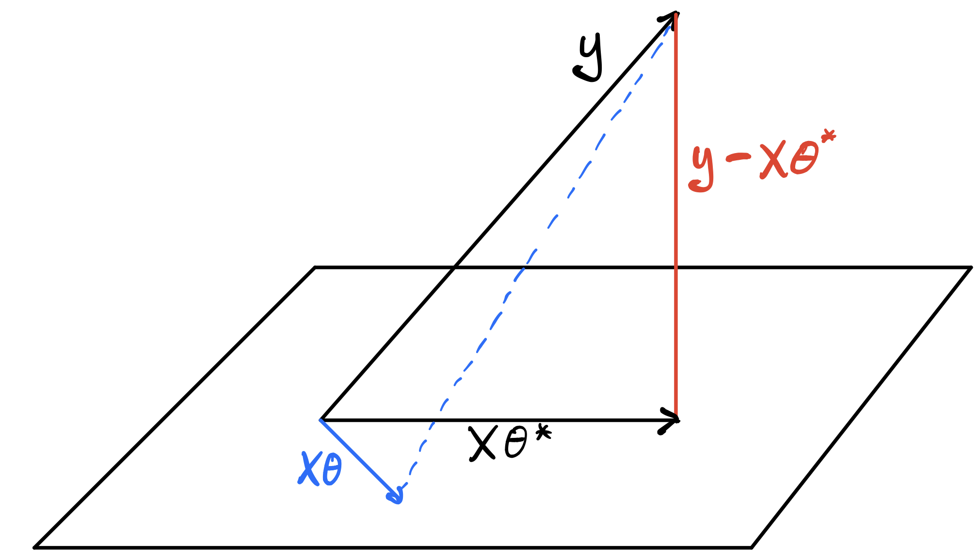
Fig. 3.2 A geometric depiction of the least squares problem.
Our goal is to minimize the \(l2\) norm of the errors, which can just be though of as the “length” of the error vectors. As you can visually see, \(\theta^*\) is optimal when the predictions \(X\theta^*\) are orthogonal to the errors. Geometrically, you can see this as if we choose some different \(\theta\), depicted in blue, the error vector gets longer. Logically, if the errors are orthogonal to the predictions, it means no change in prediction space can bring us closer to the labels \(y\). Thus, a new condition for optimality is that the errors \(y - X\theta\) are orthogonal to column space of \(X\), the space of possible predictions.
Definition: Orthogonality Two vectors \(u, v\) are orthogonal if there dot-product is zero: \(u^\top v = 0\). For a vector \(v\) to be orthogonal to \(\text{ColSp}(X)\), it must be that each column of the matrix \(X\) is orthogonal to the vector \(v\). Why? each member of column space of \(X\) can be written as a linear combination of vectors: \(Xc = u_1 c_1 + \dots u_k c_k\) where \(u_i\) is the \(i\)th column of \(X\). If \(u_i^\top v = 0\) for all \(i\), then no matter the constants \(c\) that I choose, \((u_1 c_1 + \dots u_k c_k)^\top v = c_1 u_1^\top v + \dots c_k u_k^\top v = 0\). This constraint can more simply be written as \(X^T v = 0\).
We can then enforce the orthogonality constraint of the errors and the column space by \(X^\top(y - X\theta) = 0\), which as you can see, directly gives us the normal equations.
3.3.3. Inverses & The Normal Equations
The normal equations tell us \(X^\top X \theta = X^\top y\), but does this have a solution? If you think about the geometric derivation, yes it always does have a solution as were just finding the point in the column space of \(X\) closest to \(y\). But is the solution always unique? No. You could imagine having a data matrix \(X\) such that two different weight vectors lead to the same prediction. As you get more and more data points and your data matrix gets larger and larger, this becomes a less likely outcome. We’ll first ignore this problem, then revisit it later.
Let’s assume there is one unique solution. We are then left with a \(X^\top X\) term on the left hand side. We cannot divide by matrices, vector spaces are only defined with scalar multiplication and vector addition, and inner product spaces only add an inner product. We however, can multiply by something called the inverse of a matrix.
Definition: Inverse The inverse of a matrix \(A\) is the matrix \(A^{-1}\) such that \(A^{-1} A = I\) and \(A A^{-1} = I\). where \(I\) is the identity matrix full of all zeros except with ones along the diagonal. By definition, only square matrices can have inverses. If a matrix has one, its inverse can be found by solving a system of equations.
By noticing that \(X^\top X\) is square, assuming it has an inverse the solution is:
However, we have just assumed that the matrix \(X^T X\) has an inverse, which it may not! A matrix doesn’t have inverse if its input space does not equal its output space. What do I mean by this? Let’s think about it in terms of functions and say that matrix multiplication is a function \(f(v) = Av\). The inverse function \(f^{-1}\) would take in \(Av\) and return \(v\) (\(f^{-1}(Xv) = X^{-1} Xv = Iv = v\)). As you probably learned in algebra, this type of inverse only exists if every input can be mapped to a unique output (and the inputs can cover the entire domain). For our matrix function, the input space is the entire vector space, let’s say its \(\mathbb{R}^k\). Clearly, this means we have an infinite number of inputs. To have a unique mapping, it then must be that the range of the function \(f\) is also equal to \(\mathbb{R}^k\), otherwise we would have two inputs that lead to the same output, and the function is not invertible. What is the range of \(f(v) = Av\)? It’s by definition the column space! Thus, our matrix is only invertible if the column space of the matrix is equal to the vector space itself. When a matrix satisfies this property, we say it is full rank and its inverse must exist.
When there are more unique data points than features in the data matrix \(X\), we can usually assume that an inverse to \(X^\top X\) exists. This goes beyond the scope of these notes, but if you are interested in learning about all the possible scenarios of least squares regression, a good starting place is the Moore-Penrose pseudo-inverse. You can find more information here.