2.1. Conditional Probability
In machine learning, we begin by observing data. Observed data gives us some understanding of the world and allows us to improve our decision making beyond random guessing. For example, let’s say I handed you a coin and asked you the chances of it landing on heads. You would probably guess 50%. Now let’s say I hand you the same coin, but this time told you that I had flipped it a hundred times and it only ever landed on tails. Your answer would likely be different. Taking it to a further extreme, let’s say you didn’t even know what a coin was – you would have no idea what so ever as you couldn’t lean on any prior knowledge about what the outcome of a fair coin toss should or shouldn’t be.
The point is, after we observe data, we live in a different probabilistic universe. Our observations must be true and have occurred, thereby eliminating outcomes that were previously possible. We integrate these observations or “givens” into our estimates using a framework called conditional probability. Let’s say we have two events \(A\) and \(B\), but the event \(B\), perhaps representing the observation of our data, has already occurred. Now we are interested in the probability that \(A\) occurs, given \(B\) has already occurred. We denote this conditional probability as \(P(A|B)\)
Definition: The conditional probably of an event \(A\) given an event \(B\) is: \begin{equation*} P(A|B) = \frac{P(A \cap B)}{P(B)} \end{equation*}
The interpretation of this is perhaps best illustrated by Figure 1.
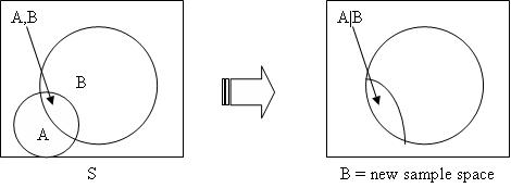
Fig. 2.1 A depiction of conditional probability.
First, we know that the event \(B\) has already occurred, meaning we can ignore the remainder of the outcome space (or sample space) that is not contained within the event \(B\) as seen on the right hand side of Figure 1. We know that \(B\) has already occurred, and now we are interested in whether or not \(A\) will occur. The probability of both happening is \(P(A \cap B)\). However, we now live in the universe of \(B\), and thus we must scale the probability of both occurring by the size of the new sample space. This directly yields the definition of conditional probability. Note that we can re-arrange the definition of conditional probability to get \(P(A \cap B) = P(A|B)P(B)\).
Let’s use our new found knowledge of conditional probability to try and make a correct decision, based off of the coin example previously discussed. Let’s say that you have a mystery coin that is fair with probability \(0.75\) and a rigged coin that always lands on heads with probability \(0.25\). We want to determine if the coin is fair or not.
Before collecting any data, we would guess that the coin is fair, as there’s a 75% chance of that happening given the information. However, were now allowed to collect some data by flipping the coin three times, and after doing so find that it lands on heads all three times. Given this new information, what’s the probability of the coin being fair?
Let \(X\) denote the number of heads observed, and \(F\) denote the event that the coin is fair. We are then interested in finding \(P(F|X=3)\). By applying the definition of conditional probability, the law of total probability, and the rearranged form of the definition of conditional probability, we get the following derivation:
\begin{equation} P(F|X=3) = \frac{P(F \cap X = 3)}{P(X = 3)} = \frac{P(X = 3 \cap F)}{P(X = 3 \cap F) + P(X = 3 \cap \bar{F})} = \frac{P(X = 3|F) P(F)}{P(X = 3|F) P(F) + P(X = 3|\bar{F}) P(\bar{F})} \end{equation}
We already know \(P(F), P(\bar{F})\) and can readily compute the remaining values. \(P(X = 3 | F) = (0.5)^3 = 0.125\), as if the coin is fair, there’s a 50% chance of it landing on heads for each toss. \(P(X = 3 \cap \bar{F}) = 1\), as if the coin is rigged to always land on heads, \(X = 3\) is the only possible outcome.
This means that \(P(F|X=3) = \frac{0.125 \times 0.75}{0.125 \times 0.75 + 0.25 \times 1} = 0.\bar{27}\). This means there is around a 27% chance that the coin is fair given the data we observed! Thus, we would guess that the coin was rigged.
The exact derivation we followed is used so often, it was promoted to theorem-hood.
Bayes Theorem: Given an event \(B\) and a set of events \(A_1, ... A_N\) that partition the sample space \(\Omega\), \begin{equation} P(A_i | B) = \frac{P(B|A_i)P(A_i)}{\sum_{j=1}^N P(B|A_j)P(A_j)} \end{equation}
We’ll see how conditional probability is particularly useful in the next section.